Tracer Tool#
The Tracer (trc) Tool computes the evolution of passive tracer and its adjoint with a user-specified initial tracer and its adjoint. The tool uses the pre-computed weekly-mean ECCO V4r4 circulation and mixing to timestep the passive tracer. For this reason, we refer to the tracer as an offline passive tracer. The wall time of the model integration is significantly reduced due to the use of pre-computed circulation and mixing.
In this tutorial, we demonstrate how to run a passive tracer initialized in the upper 10 m of the Niño 3.4 region (5°S-5°N, 170°W-120°W) from day 35 to day 365. We then show how to plot some of the results. Whether the run is for a tracer or its adjoint is determined by how the start day and end day are set. If the start day (35 in this example) is earlier than the end day (365), it is a forward tracer. Its adjoint can be run using the same parameters, except with the start day set to 365 and the end day set to 35.
Run Tracer Tool#
We start EMU (see, e.g., Adjoint Tool) and choose the Tracer Tool by entering 5.
choice is 5) Tracer Tool (trc)
See /efs_ecco/ECCO/EMU/emu_userinterface_dir/README_trc

************************************
    EMU Tracer Tool (singularity)
************************************

**** Step 1: Tool Setup
     Running setup_trc.sh

... Setting up ECCO V4r4 Passive Tracer Tool ...


**** Step 2: Specification
     Running trc.x

Passive Tracer Tool ...

 Define passive tracer distribution ...

------------------
Enter START and END days of integration ...
(days between 1 and 9485)
(   1 being 02 January  1992)
(9485 being 20 December 2017)

   Tool computes forward tracer when START lt END and
   adjoint tracer when START gt END.
We enter 35 for the start day.
Enter end day ... (1-9485)?
And enter 365 for the end day.
Start and End days =  35 365

---------------------------------
   Forward tracer computation
---------------------------------

Enter tracer at start time ...
Choose either a unit tracer at a point (1) or
one with 3d distribution (2) ... (1/2)?
We are now prompted to set the initial tracer. We will enter 2 to set the tracer with a 3D distribution and then enter 1 to interactively set the spatial range of the initial distribution. We want to set the initial distribution in the upper 10 m of the Niño 3.4 region (5°S-5°N, 170°W-120°W). Accordingly, we enter -170, -120, -5, 5, 10, and 0. The configuration is now complete.
Choose either a unit tracer at a point (1) or
one with 3d distribution (2) ... (1/2)?
2
   ... Initial tracer has 3d distribution
   Interactively specify initial tracer (1) or read from user file (2) ... (1/2)?
1

    Interactively creating initial TRC.
 Enter west most longitude (-180E to 180E)... x1?
-170
 Enter east most longitude (-180E to 180E)... x2?
    (choose x2=x1 for zonally global volume)
-120
 Enter south most latitude (-90N to 90N)... y1?
-5
 Enter north most latitude (-90N to 90N)... y2?
5
 Enter deepest depth (0-6000m) ... z1?
10
 Enter shallowest depth (0-6000m)... z2?
0
   3d tracer output:

   trc3d.-170.0_-120.0_-5.0_5.0_10.0_0.0


Tracer Tool output will be in : emu_trc_35_365_trc3d.-170.0_-120.0_-5.0_5.0_10.0_0.0

... Done trc setup

**** Step 3: Calculation
  1) Set up files for tracer integration
     Running do_trc_prep.sh

diags exists
  2) Integrate tracer
     submitting pbs_trc.sh

... Running batch job pbs_trc.sh
    to compute passive tracer evolution.

    Estimated wallclock time:
#SBATCH --ntasks-per-node=36

********************************************
    Results will be in  emu_trc_35_365_trc3d.-170.0_-120.0_-5.0_5.0_10.0_0.0/output
********************************************

Progress of the computation can be monitored by
  ls -l emu_trc_35_365_trc3d.-170.0_-120.0_-5.0_5.0_10.0_0.0/temp/diags/ptracer_mon_mean*data | wc -l
which counts the number of monthly mean tracer output files
until completion when directory diags will be moved and this
command will return an error (No such file or directory)
and list zero as the count.

Submitted batch job 824

EMU interactive execution complete. Fri Oct  4 16:43:45 UTC 2024
The run name is emu_trc_35_365_trc3d.-170.0_-120.0_-5.0_5.0_10.0_0.0. The run should take roughly 20 minutes to finish.
Visualize Tracer Tool Results#
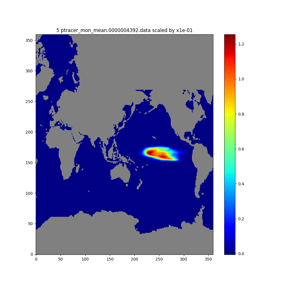
We will create maps of depth-integrated tracer contents at month 2 and month 5.
Tip
A Jupyter Notebook, trc_viz (after downloading, rename it to trc_viz.ipynb), is provided for users’ convenience. It reproduces the steps and figures described in this visualization tutorial. Users can also add more sophisticated analysis on top of this notebook.
Same as in Sampling Tool, we first log into OSS and start a Jupyter Notebook session.
Method 2: Argument-based Input#
The detailed steps for Method 2 can be found in trc_viz.ipynb (see Tip above).
Load modules
import sys
sys.path.append('/efs_ecco/ECCO/EMU/emu_userinterface_dir/')
import numpy as np
import os
import matplotlib.pyplot as plt
import lib_python
import plot_adj
Invoke Method 2
globals_dict = ept.emu_plot(run_name="/efs_ecco/owang/ECCO/EMU/tryout/emu_trc_35_365_trc3d.-170.0_-120.0_-5.0_5.0_10.0_0.0",
                            avg_type='m',
                            pfile_beg=0, pfile_end=1000000)
Found file: /efs_ecco/ECCO/EMU/emu_userinterface_dir/emu_env.singularity
EMU Input Files directory: /efs/owang/ECCO/EMU_test/emu_input_dir

Specified directory of EMU run to examine: /efs_ecco/owang/ECCO/EMU/tryout/emu_trc_35_365_trc3d.-170.0_-120.0_-5.0_5.0_10.0_0.0

Reading /efs_ecco/owang/ECCO/EMU/tryout/emu_trc_35_365_trc3d.-170.0_-120.0_-5.0_5.0_10.0_0.0

Reading Tracer Tool output ...

Detected     11 files of ptracer_mon_mean.*.data
Detected     10 files of ptracer_mon_snap.*.data

Averaging type ("m" for monthly or "s" for snapshot): m

==> Reading and plotting monthly means ...
Specified start and end files #: 0 and 1000000


Reading file ... /efs_ecco/owang/ECCO/EMU/tryout/emu_trc_35_365_trc3d.-170.0_-120.0_-5.0_5.0_10.0_0.0/output/ptracer_mon_mean.0000001464.data

Reading file ... /efs_ecco/owang/ECCO/EMU/tryout/emu_trc_35_365_trc3d.-170.0_-120.0_-5.0_5.0_10.0_0.0/output/ptracer_mon_mean.0000002196.data

Reading file ... /efs_ecco/owang/ECCO/EMU/tryout/emu_trc_35_365_trc3d.-170.0_-120.0_-5.0_5.0_10.0_0.0/output/ptracer_mon_mean.0000002928.data

Reading file ... /efs_ecco/owang/ECCO/EMU/tryout/emu_trc_35_365_trc3d.-170.0_-120.0_-5.0_5.0_10.0_0.0/output/ptracer_mon_mean.0000003660.data

Reading file ... /efs_ecco/owang/ECCO/EMU/tryout/emu_trc_35_365_trc3d.-170.0_-120.0_-5.0_5.0_10.0_0.0/output/ptracer_mon_mean.0000004392.data

Reading file ... /efs_ecco/owang/ECCO/EMU/tryout/emu_trc_35_365_trc3d.-170.0_-120.0_-5.0_5.0_10.0_0.0/output/ptracer_mon_mean.0000005124.data

Reading file ... /efs_ecco/owang/ECCO/EMU/tryout/emu_trc_35_365_trc3d.-170.0_-120.0_-5.0_5.0_10.0_0.0/output/ptracer_mon_mean.0000005856.data

Reading file ... /efs_ecco/owang/ECCO/EMU/tryout/emu_trc_35_365_trc3d.-170.0_-120.0_-5.0_5.0_10.0_0.0/output/ptracer_mon_mean.0000006588.data

Reading file ... /efs_ecco/owang/ECCO/EMU/tryout/emu_trc_35_365_trc3d.-170.0_-120.0_-5.0_5.0_10.0_0.0/output/ptracer_mon_mean.0000007320.data

Reading file ... /efs_ecco/owang/ECCO/EMU/tryout/emu_trc_35_365_trc3d.-170.0_-120.0_-5.0_5.0_10.0_0.0/output/ptracer_mon_mean.0000008052.data

Reading file ... /efs_ecco/owang/ECCO/EMU/tryout/emu_trc_35_365_trc3d.-170.0_-120.0_-5.0_5.0_10.0_0.0/output/ptracer_mon_mean.0000008748.data

*********************************************
Returning variable
   return_vars_tmp, a dictionary with one item being
   trc: last plotted tracer (3d) or time series of tracer (3d)


***********************
EMU variables read as global variables in module global_emu_var (emu); e.g., emu.nx
***********************
cs                  drc                 drf                 dvol3d
dxc                 dxg                 dyc                 dyg
hfacc               hfacs               hfacw               nr
nx                  ny                  rac                 ras
raw                 raz                 rc                  rf
sn                  trc3d               xc                  xg
yc                  yg
Extract Data from Return Dictionary
trc_all = return_vars_dict['trc'] # 3d tracer content
trc_all_vsum = np.sum(hfacc * np.expand_dims(drf, axis=(1,2)) * trc_all, axis=1)
files = return_vars_dict['files']
Make plot First set some parameters for plot and then make plots.
# set some plotting parameters
dscale = 0.1
cmap = plt.cm.jet
cmap.set_bad(color='gray')  # Set the color for masked elements to gray
# Tracer at month 2
plt.figure(figsize=(10,10))
imon = 2

fname=os.path.basename(files[imon-1])
ftitle = f'{imon} {fname} scaled by x{dscale:.0e}'
# Apply the scaling factor and mask out the land points
masked_dumg = dscale*lib_python.nat2globe(trc_all_vsum[imon-1,:])
dummskg = lib_python.nat2globe(hfacc[0])
masked_dumg[dummskg==0]=np.nan

plt.title(ftitle)
plt.imshow(masked_dumg, origin='lower',cmap=cmap, aspect='auto')
plt.colorbar()
plt.show()

# Tracer at month 5
plt.figure(figsize=(10,10))
imon = 5
fname=os.path.basename(files[imon-1])
ftitle = f'{imon} {fname} scaled by x{dscale:.0e}'
# Apply the scaling factor and mask out the land points
masked_dumg = dscale*lib_python.nat2globe(trc_all_vsum[imon-1,:])
dummskg = lib_python.nat2globe(hfacc[0])
masked_dumg[dummskg==0]=np.nan

plt.title(ftitle)
plt.imshow(masked_dumg, origin='lower',cmap=cmap, aspect='auto')
plt.colorbar()
plt.show()
Method 2 generates the same two figures (not shown; see the figures embedded in trc_viz.ipynb) as those generated by Method 1.


