Attribution Tool#
The Attribution (atrb) Tool evaluates model state time-series by control type.
In this tutorial, we demonstrate how to use the Attribution Tool to evaluate the time-series of temperature (theta, in deg C) of the upper 10 m of the Niño 3.4 region (5°S-5°N, 170°W-120°W). We then show how to plot some of the results.
Run Attribution Tool#
Request an Interactive Node#
The Attribution Tool is one of two tools typically run as a shell script without being submitted as a batch job (see EMU Introduction). As described in EMU Introduction, we first request an interactive node:”
salloc --ntasks=2 --ntasks-per-node=2 --partition=sealevel-c5xl-demand --time=01:00:00
Once the requested node is available (see Reproducing ECCO Version 4 Release 4 for examples on how to use squeue to check job status), we proceed with running the tool.
Configure and Run Attribution Tool#
We start EMU (see, e.g., Adjoint Tool) and choose the Attribution Tool by entering 8.
8
choice is 8) Attribution Tool (atrb)
See /efs_ecco/ECCO/EMU/emu_userinterface_dir/README_atrb

************************************
    EMU Attribution Tool (singularity)
************************************

**** Steps 1 & 2: Setup & Specification


Evaluating model time-series ...

 Define objective function (OBJF) ...
 Available VARIABLES are ...
    1) SSH (m)
    2) OBP (equivalent sea level m)
    3) THETA (deg C)
    4) SALT (PSU)
    5) UV (m/s)

   Monthly or Daily mean ... (m/d)?
   (NOTE: daily mean available for SSH and OBP only.)
We then choose monthly mean by entering m.
   fmd = m
   ==> Sampling MONTHLY means ...

------------------
   Choose OBFJ variable (v in Eq 1 of Guide) # 1 ... (1-5)?
   (Enter 0 to end variable selection)
We enter 3 to select THETA (deg C) and 2 to choose the option of “VARIABLE weighted in space”.
3
   OBJF variable  1 is THETA
 Choose either VARIABLE at a point (1) or  VARIABLE weighted in space (2) ... (1/2)?
2
 ... OBJF will be a linear function of selected variable
    i.e., MULT * SUM( MASK * VARIABLE )

   Interactively specify MASK (1) or read from user file (2) ... (1/2)?
We then choose to interactively define the mask by entering 1 and specify the spatial range for the the Niño 3.4 box: -170, -120, -5, 5, 10, and 0, as done in the Tracer Tool.
1

    Interactively creating MASK for volume mean.

 Enter west most longitude (-180E to 180E)... x1?
-170
 Enter east most longitude (-180E to 180E)... x2?
    (choose x2=x1 for zonally global volume)
-120
 Enter south most latitude (-90N to 90N)... y1?
-5
 Enter north most latitude (-90N to 90N)... y2?
5
 Enter deepest depth (0-6000m) ... z1?
10
 Enter shallowest depth (0-6000m)... z2?
0
We are then prompted with the following:
Should volume mean be relative to global mean ... (enter 1 for yes)?
We choose not to make the volume mean relative to the global mean by entering 0.
   3d Mask output:

   mask3d.-170.0_-120.0_-5.0_5.0_10.0_0.0

   Enter scaling factor (alpha in Eq 1 of Guide)... ?
We then enter 1 for the scaling factor.
amult =   1.0000E+00

------------------
   Choose OBFJ variable (v in Eq 1 of Guide) # 2 ... (1-5)?
   (Enter 0 to end variable selection)
We enter 0 to end the selection and the evaluation starts.
Done interactive specification.
Begin evaluating time-series ...

Tool output will be in: emu_atrb_m_3_mask3d.-170.0_-120.0_-5.0_5.0_10.0_0.0_1

Sampling reference run ...
from:  /emu_input_dir/emu_ref/diags

Sampling time-mean wind run ...
from:  /emu_input_dir/emu_msim/mean_oceTAUX_oceTAUY/diags

Sampling time-mean heat flux run ...
from:  /emu_input_dir/emu_msim/mean_TFLUX_oceQsw/diags

Sampling time-mean freshwater flux run ...
from:  /emu_input_dir/emu_msim/mean_oceFWflx/diags
^[c
Sampling time-mean salt flux run ...
from:  /emu_input_dir/emu_msim/mean_oceSflux_oceSPflx/diags

Sampling time-mean pressure load run ...
from:  /emu_input_dir/emu_msim/mean_sIceLoadPatmPload_nopabar/diags

Sampling time-mean initial condition run ...
from:  /emu_input_dir/emu_msim/mean_IC/diags

Computing individual control contribution ...

********************************************
    Done. Results are in /efs_ecco/owang/ECCO/EMU/tryout/emu_atrb_m_3_mask3d.-170.0_-120.0_-5.0_5.0_10.0_0.0_1/output
********************************************


EMU interactive execution complete. Fri Oct  4 22:56:04 UTC 2024
The run name is emu_atrb_m_3_mask3d.-170.0_-120.0_-5.0_5.0_10.0_0.0_1.
Visualize Adjoint Tool Results#
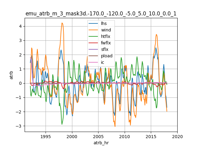
We now demonstrate how to visualize the Attribution Tool results: the tendency term of the quantity of interest, as well as contributions from controls, including atmospheric forcing and initial conditions. Plotting the results of Modified Simulation Tool is the same as plotting Sampling Tool results, except that we now enter or specify the run directory name: /efs_ecco/owang/ECCO/EMU/tryout/emu_atrb_m_3_mask3d.-170.0_-120.0_-5.0_5.0_10.0_0.0_1. Again, we will show two methods of using the visualization tool.
Tip
A Jupyter Notebook, atrb_viz (after downloading, rename it to atrb_viz.ipynb), is provided for users’ convenience. It reproduces the steps and figures described in this visualization tutorial. Users can also add more sophisticated analysis on top of this notebook.
Same as in Sampling Tool, we first log into OSS and start a Jupyter Notebook session.
Method 2: Argument-based Input#
The detailed steps for Method 2 can be found in atrb_viz.ipynb (see Tip above).
Load modules
import sys
sys.path.append('/efs_ecco/ECCO/EMU/emu_userinterface_dir/')
import emu_plot_arg_py as ept
import plt_atrb
Invoke Method 2
# Attribution Tool
globals_dict = ept.emu_plot(run_name="/efs_ecco/owang/ECCO/EMU/tryout/emu_atrb_m_3_mask3d.-170.0_-120.0_-5.0_5.0_10.0_0.0_1")
Found file: /efs_ecco/ECCO/EMU/emu_userinterface_dir/emu_env.singularity
EMU Input Files directory: /efs/owang/ECCO/EMU_test/emu_input_dir

Specified directory of EMU run to examine: /efs_ecco/owang/ECCO/EMU/tryout/emu_atrb_m_3_mask3d.-170.0_-120.0_-5.0_5.0_10.0_0.0_1

Reading /efs_ecco/owang/ECCO/EMU/tryout/emu_atrb_m_3_mask3d.-170.0_-120.0_-5.0_5.0_10.0_0.0_1

Reading Attribution Tool output ...
*********************************************
Read OBJF and contributions to it from different controls
   atrb: temporal anomaly
   atrb_mn: reference time-mean
   fctrl: names of atrb/atrb_mn variables
from file /efs_ecco/owang/ECCO/EMU/tryout/emu_atrb_m_3_mask3d.-170.0_-120.0_-5.0_5.0_10.0_0.0_1/output/atrb.out_312

*********************************************
Read variable
   atrb_hr: sample time (hours from 1/1/1992 12Z)
from file /efs_ecco/owang/ECCO/EMU/tryout/emu_atrb_m_3_mask3d.-170.0_-120.0_-5.0_5.0_10.0_0.0_1/output/atrb.step_312


***********************
EMU variables read as global variables in module global_emu_var (emu); e.g., emu.nx
***********************
atrb                atrb_ctrl           atrb_hr             atrb_mn
cs                  drc                 drf                 dvol3d
dxc                 dxg                 dyc                 dyg
hfacc               hfacs               hfacw               nr
nx                  ny                  rac                 ras
raw                 raz                 rc                  rf
sn                  xc                  xg                  yc
yg
Extract Data from Return Dictionary
# Extract return dictionary
return_vars_dict = globals_dict.get('return_vars')
Make plot
# Extract data for the plot
atrb_t = return_vars_dict['time_values']
atrb = return_vars_dict['variable']
fctrl = return_vars_dict['ctrl_name']
frun_file = return_vars_dict['plot_title']
nterms = len(fctrl)
fld_all = return_vars_dict['variable']

# Create plot
plot_atrb.create_atrb_fig(atrb_t, atrb, frun_file, fctrl, nterms)
Method 2 generates the same figure (not shown; see the figure embedded in atrb_viz.ipynb) as that generated by Method 1.


