Convolution Tool#
The Convolution (conv) Tool conducts adjoint-based decomposition of the quantity of interest (QoI). It convolves adjoint gradients (such as those computed in the Adjoint Tool) with control changes to decompose the contributions to QoI changes as a function of control type, space, and time lag.
Run Convolution Tool#
We start EMU (see, e.g., Adjoint Tool) and choose the Convolution Tool by entering 4.
choice is 4) Convolution Tool (conv)
See /efs_ecco/ECCO/EMU/emu_userinterface_dir/README_conv

************************************
    EMU Convolution Tool (singularity)
************************************

**** Step 1 & 2: Setup & Specification

Specify directory name of Adjoint Tool output or its equivalent
where the adjoint gradients to use in the convolution are.
Files must have the same name and format as those of the
Adjoint Tool, in a directory named 'output' with its parent
directory having prefix 'emu_adj';
  e.g., emu_adj_SOMETHING/output

Enter directory name with the adjoint gradients ... ?
We are prompted to enter the directory name with the adjoint gradients, which can be from an Adjoint Tool run. We will use the adjoint gradients computed in the Adjoint Tool tutorial, which is /efs_ecco/owang/ECCO/EMU/tryout/emu_adj_6_6_2_45_585_1/output, the output directory for the Adjoint Tool run emu_adj_6_6_2_45_585_1 (see EMU Introduction for an explanation of the output directory). After that, we need to choose what forcings (i.e., controls) to use for the convolution.
     Running conv.x
Convolution Tool ...

Specify forcing, adjoint gradient, and maximum lag below ...

 f_inputdir : /efs_ecco/ECCO/EMU/emu_input_dir
 f_adxx : /efs_ecco/owang/ECCO/EMU/tryout/emu_adj_6_6_2_45_585_1/output
 f_adxx_read : /inside_alt
V4r4 weekly forcing is in directory
     /efs_ecco/ECCO/EMU/emu_input_dir/forcing/other/flux-forced/forcing_weekly

Use V4r4's weekly forcing for convolution (phi in Eq 7 of Guide) ... (Y/N)?
We choose to use V4r4’s weekly by entering y.
Reading forcing from directory
     /efs_ecco/ECCO/EMU/emu_input_dir/forcing/other/flux-forced/forcing_weekly

     Reading adxx from
     /efs_ecco/owang/ECCO/EMU/tryout/emu_adj_6_6_2_45_585_1/output

     number of adxx records = 29

     Zero lag at (weeks) = 27

Enter maximum lag (weeks) to use in convolution (delta_t_max in Eq 7 of Guide) ... (0-26)?
We are now prompted to enter the maximum lag (in weeks) to use in the convolution. Note that the tool determines a range of lags based on the adjoint gradients, which is between 0 and 26 weeks, as shown in the on-screen message above. We choose the maximum lag to be 26. With that, the configuration of the Convolution Tool is complete, and a batch job is submitted.
     nlag =  26

Convolution Tool output will be in : emu_conv_6_6_2_45_585_1_26

... Done conv setup (conv.out)

*********************************
    Run "do_conv.x" to conduct convolution.
*********************************


**** Step 3: Calculation
     Running do_conv.x

... Running batch job pbs_conv.sh
    to compute the convolution.

    Estimated wallclock time:
#SBATCH --ntasks-per-node=36

********************************************
    Results will be in  emu_conv_6_6_2_45_585_1_26/output
********************************************

Submitted batch job 823

EMU interactive execution complete. Fri Oct  4 00:51:54 UTC 2024
Visualize Convolution Tool Results#
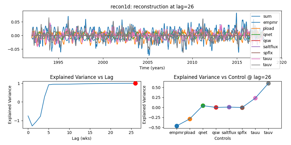
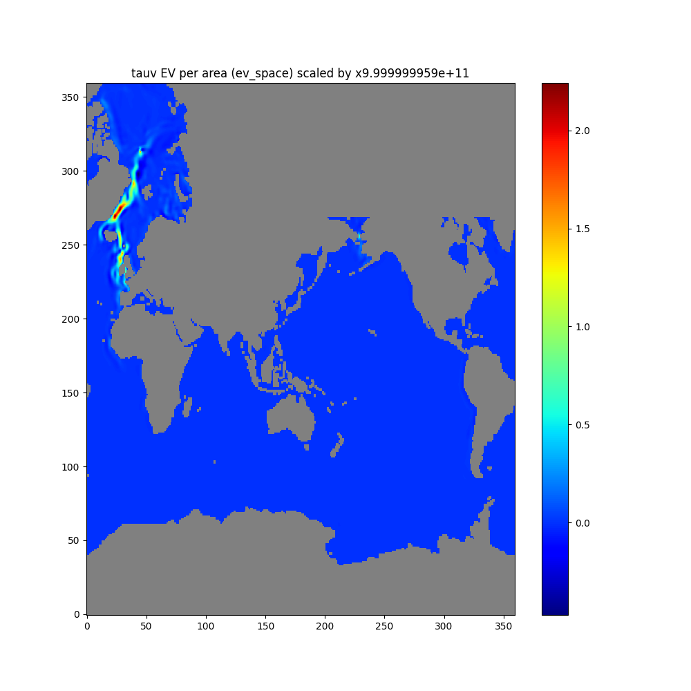
Based on the Convolution Tool results, we will plot the reconstructed time series, explained variance versus time lag (in weeks), and explained variance versus control. Additionally, we will create an example plot of explained variance versus space.
Plotting the results of the Convolution Tool is the same as plotting Sampling Tool results, except that we now enter the run directory emu_conv_6_6_2_45_585_1_26. Again, we will show two methods of using the visualization tool.
Tip
A Jupyter Notebook, conv_viz (after downloading, rename it to conv_viz.ipynb), is provided for users’ convenience. It reproduces the steps and figures described in this visualization tutorial. Users can also add more sophisticated analysis on top of this notebook.
Same as in Sampling Tool, we first log into OSS and start a Jupyter Notebook session.
Method 2: Argument-based Input#
The detailed steps for Method 2 can be found in conv_viz.ipynb (see Tip above).
Load modules
import sys
sys.path.append('/efs_ecco/ECCO/EMU/emu_userinterface_dir/')
import emu_plot_arg_py as ept
import numpy as np
import matplotlib.pyplot as plt
import lib_python
import plot_conv
import plot_conv_sub
Invoke Method 2
globals_dict = ept.emu_plot(run_name="/efs_ecco/owang/ECCO/EMU/tryout/emu_conv_6_6_2_45_585_1_26",
expvar_space='y');
Found file: /efs_ecco/ECCO/EMU/emu_userinterface_dir/emu_env.singularity
EMU Input Files directory: /efs/owang/ECCO/EMU_test/emu_input_dir
Specified directory of EMU run to examine: /efs_ecco/owang/ECCO/EMU/tryout/emu_conv_6_6_2_45_585_1_26
Reading /efs_ecco/owang/ECCO/EMU/tryout/emu_conv_6_6_2_45_585_1_26

Reading Convolution Tool output ...
<_io.BufferedReader name='/efs_ecco/owang/ECCO/EMU/tryout/emu_conv_6_6_2_45_585_1_26/output/recon1d_empmr.data'>
<_io.BufferedReader name='/efs_ecco/owang/ECCO/EMU/tryout/emu_conv_6_6_2_45_585_1_26/output/recon1d_pload.data'>
<_io.BufferedReader name='/efs_ecco/owang/ECCO/EMU/tryout/emu_conv_6_6_2_45_585_1_26/output/recon1d_qnet.data'>
<_io.BufferedReader name='/efs_ecco/owang/ECCO/EMU/tryout/emu_conv_6_6_2_45_585_1_26/output/recon1d_qsw.data'>
<_io.BufferedReader name='/efs_ecco/owang/ECCO/EMU/tryout/emu_conv_6_6_2_45_585_1_26/output/recon1d_saltflux.data'>
<_io.BufferedReader name='/efs_ecco/owang/ECCO/EMU/tryout/emu_conv_6_6_2_45_585_1_26/output/recon1d_spflx.data'>
<_io.BufferedReader name='/efs_ecco/owang/ECCO/EMU/tryout/emu_conv_6_6_2_45_585_1_26/output/recon1d_tauu.data'>
<_io.BufferedReader name='/efs_ecco/owang/ECCO/EMU/tryout/emu_conv_6_6_2_45_585_1_26/output/recon1d_tauv.data'>
*********************************************
Read variable recon1d, the global spatial sum time-series
of the convolution as a function of lag and control.
   recon1d: adjoint gradient reconstruction
from file recon1d_*.data

*********************************************
Read variable
   istep: time (hours since 1/1/1992 12Z) of recon1d
from file istep_empmr.data

Minimum year: 1991
Maximum year: 2020
*********************************************
Computed Explained Variance (EV) vs lag with all controls.
   ev_lag: EV as function of lag

*********************************************
Computed Explained Variance (EV) vs control at maximum lag.
   ev_ctrl: EV as function of control
Reading recon2d_*.data and computing explained variance vs space (ev_space) ...
Variable recon2d is the adjoint gradient reconstruction (time-series)
as a function of space by a particular control using the maximum lag
chosen in the convolution. Here, recon2d is read to compute the explained
variance vs space (ev_space), but recon2d is not retained by this plotting
routine to minimize memory usage.
*********************************************
Detected ev_space file. Reading explained variance (EV)
as a function of space and control with respect to
the variance of full reconstruction up to maximum lag.
ev_space: EV per unit area
from file
/efs_ecco/owang/ECCO/EMU/tryout/emu_conv_6_6_2_45_585_1_26/output/plot_conv_recon2d.ev_space
Plot explained variance vs space (ev_space) ...
***********************
EMU variables read as global variables in module global_emu_var (emu); e.g., emu.nx
***********************
cs drc drf dvol3d
dxc dxg dyc dyg
ev_ctrl ev_lag ev_space hfacc
hfacs hfacw istep nr
nx ny rac ras
raw raz rc recon1d
rf sn xc xg
yc yg
Extract Data from Return Dictionary
return_vars_dict = globals_dict.get('return_vars')
hfacc = globals_dict.get('emu').hfacc

ww = return_vars_dict['time_values']
recon1d_sum = return_vars_dict['recon1d_sum_all_ctrl_vs_lag_time']
wwmin = return_vars_dict['time_values_min']
wwmax = return_vars_dict['time_values_max']
nctrl = return_vars_dict['num_ctrl']
recon1d = return_vars_dict['recon1d_vs_lag_time']
fctrl = return_vars_dict['ctrl_name']
tlag = return_vars_dict['lag_in_weeks']
ev_lag = return_vars_dict['expvar_vs_lag']
tctrl = return_vars_dict['ctrl_idx']
ev_ctrl = return_vars_dict['expvar_vs_ctrl']
nlag = return_vars_dict['num_lag_in_weeks']
tctrl_min = return_vars_dict['ctrl_idx_min']
tctrl_max = return_vars_dict['ctrl_idx_max']
ev_space = return_vars_dict['expvar_vs_space']
Make plot First set some parameters for plot and then make plots.
# Set up parameters for plots
ip = 26 # lag
frun = '/efs_ecco/owang/ECCO/EMU/tryout/emu_conv_6_6_2_45_585_1_26'
ic = 8 # for adxx_tauv
dscale = 1e12 # scaling factor
# Apply the scaling factor and mask out the land points
masked_dumg = dscale*lib_python.nat2globe(ev_space[ic-1,:])
dummskg = lib_python.nat2globe(hfacc[0])
masked_dumg[dummskg==0]=np.nan

cmap = plt.cm.jet
cmap.set_bad(color='gray')  # Set the color for masked elements to gray

# Line plots
plot_conv.plot_conv_lin(ip, ww, recon1d_sum, wwmin, wwmax,
                  nctrl, recon1d, fctrl,
                  tlag, ev_lag,
                  tctrl, ev_ctrl, nlag, tctrl_min, tctrl_max)

# Explained variance vs. space
plt.figure(figsize=(10,10))
ftitle = f"{fctrl[ic -1]} EV per area (ev_space) scaled by x{dscale:.9e}"
plt.title(ftitle)
plt.imshow(masked_dumg, origin='lower',cmap=cmap, aspect='auto')
plt.colorbar()
Method 2 generates the same two figures (not shown; see the figures embedded in conv_viz.ipynb) as those generated by Method 1.


 We exit the plotting tool by entering