Adjoint Tool#
The Adjoint (adj) Tool computes the model state’s adjoint gradients with respect to different controls. These gradients can be used in the Convolution Tool to conduct adjoint-based reconstruction and decomposition of the quantity of interest.
Run Adjoint Tool#
Similar to Forward Gradient (fgrd) Tool, after setup the Adjoint Tool will be automatically submitted as a SLURM batch job; there is no need to request an interactive node.
In this example, we want to use the Adjoint Tool to compute the gradients of the monthly-mean OBP in June 1992 at one model grid with respect to the controls.
**Starting emu script, **
/efs_ecco/ECCO/EMU/emu_userinterface_dir/emu
From the list of tools, we choose Adjoint Tool by entering 3.
choice is 3) Adjoint Tool (adj)
See /efs_ecco/ECCO/EMU/emu_userinterface_dir/README_adj

************************************
    EMU Adjoint Tool  (singularity)
************************************

**** Step 1: Tool Setup
     Running setup_adj.csh

... Setting up ECCO V4r4 Adjoint Tool ...


**** Step 2: Specification
     Running adj.x

Define objective function (OBJF; J^bar in Eq 5 of Guide) ...

First define OBJF time-period (t_start and t_g in Eq 6 of Guide) ...

   V4r4 can integrate from 1/1/1992 12Z to 12/31/2017 12Z
       which is 26-years (312-months).

   Select FIRST and LAST month of OBJF averaging period.
   Enter FIRST month of OBJF period (t_start in Eq 6 of Guide) ... (1-312)?
We enter 6 for the first month of the OBJF period, which is June 1992, as the model starts on January 1, 1992.
Enter LAST month of OBJF period (t_g in Eq 6 of Guide) ... (1-312)?
We enter 6 for the last month.
   PERIOD start & end months = 6 6

   ... Program has set computation periods in files data and pbs_adj.sh accordingly.
   ... Estimated wallclock hours is    4

Next define OBJF variable(s) (v in Eq 1 of Guide) ...

   Available VARIABLES are ...
    1) SSH (m)
    2) OBP (equivalent sea level m)
    3) THETA (deg C)
    4) SALT (PSU)
    5) UV (m/s)

------------------
   Choose OBFJ variable (v in Eq 1 of Guide) # 1 ... (1-5)?
   (Enter 0 to end variable selection)
We select OBP by entering 2.
   OBJF variable  1 is OBP
   Choose either VARIABLE at a point (1) or VARIABLE weighted in space (2) ... (1/2)?
We enter 1 to choose OBP at one grid point. We further enter 1 to select a native grid location and provide the model grid i and j indices by enter 45 and 585. This grid point is at the North Pole. We then choose to have the OBP value relative to its global mean by entering 1. We set the scaling factor to one by enter 1. Finally, we end the variable selection by enter 0. These few steps are the same as those in other tools, so the on-screen messages are not repeated here.
After ending the variable selection, we will see the following message.
Adjoint Tool output will be in : emu_adj_6_6_2_45_585_1

Wrote adj.dir_out
**** Step 3: Calculation
  1) Set up files for MITgcm
diags exists
diags exists
diags exists
diags exists
diags exists
diags exists
diags exists
diags exists
diags exists
diags exists
diags exists
diags exists
diags exists
diags exists
diags exists
diags exists
diags exists
diags exists
diags exists
diags exists
diags exists
  2) Run MITgcm adjoint
... Running batch job pbs_adj.sh
    to compute the model's adjoint gradients.

    Estimated wallclock time:
#SBATCH --ntasks-per-node=36

********************************************
    Results will be in  /efs_ecco/owang/ECCO/EMU/tryout/emu_adj_6_6_2_45_585_1/output
********************************************

Progress of the computation can be monitored by
  grep ad_time_tsnumber /efs_ecco/owang/ECCO/EMU/tryout/emu_adj_6_6_2_45_585_1/temp/STDOUT.0000
which lists the model's time-step (one-hour) at 10-day
intervals backward from the target instant to the model's
initial time (hour 0), 01 January 1992 12Z.

Submitted batch job 821

EMU interactive execution complete. Thu Oct  3 17:19:10 UTC 2024
The job has been submitted as a batch job with the job ID 821. The job should take less than 3 hours to complete on the P-Cluster.
Visualize Adjoint Tool Results#
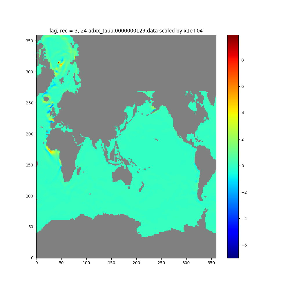
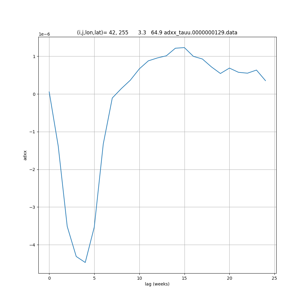
For the results of the Adjoint Tool, the built-in EMU plotting tool can plot maps of gradients at a select lag and time-series of gradients at a select location vs. lag.
Plotting the results of Adjoint Tool is the same as plotting Sampling Tool results, except that we now enter the run directory emu_adj_6_6_2_45_585_1. Again, we will show two methods of using the visualization tool.
Tip
A Jupyter Notebook, adj_viz (after downloading, rename it to adj_viz.ipynb), is provided for users’ convenience. It reproduces the steps and figures described in this visualization tutorial. Users can also add more sophisticated analysis on top of this notebook.
Same as in Sampling Tool, we first log into OSS and start a Jupyter Notebook session.
Method 2: Argument-based Input#
The detailed steps for Method 2 can be found in adj_viz.ipynb (see Tip above).
Load modules
import sys
sys.path.append('/efs_ecco/ECCO/EMU/emu_userinterface_dir/')
import emu_plot_arg_py as ept
import numpy as np
import matplotlib.pyplot as plt
import lib_python
import plot_adj
Invoke Method 2
globals_dict = ept.emu_plot(run_name="/efs_ecco/owang/ECCO/EMU/tryout/emu_adj_6_6_2_45_585_1",
                            ctrl_num_list=[1, 2, 3, 4, 5, 6, 7, 8],
                            lag_beg=0, lag_end=1000000);
Found file: /efs_ecco/ECCO/EMU/emu_userinterface_dir/emu_env.singularity
EMU Input Files directory: /efs/owang/ECCO/EMU_test/emu_input_dir

Specified directory of EMU run to examine: /efs_ecco/owang/ECCO/EMU/tryout/emu_adj_6_6_2_45_585_1

Reading /efs_ecco/owang/ECCO/EMU/tryout/emu_adj_6_6_2_45_585_1

Reading Adjoint Tool output ...

Found file: adxx_empmr.0000000129.data

*********************************************
Read adjoint gradient for empmr
   adxx: adjoint gradient as a function of space and lag
from file /efs_ecco/owang/ECCO/EMU/tryout/emu_adj_6_6_2_45_585_1/output/adxx_empmr.0000000129.data

Zero lag at (week/record) = 27
Max  lag at (week/record) = 1
Specified start and end files #: 0 and 1000000

*********************************************
Outputting adxx_empmr

Found file: adxx_pload.0000000129.data

# ... output for other controls omitted for brevity ...

*********************************************
Read adjoint gradient for tauv
   adxx: adjoint gradient as a function of space and lag
from file /efs_ecco/owang/ECCO/EMU/tryout/emu_adj_6_6_2_45_585_1/output/adxx_tauv.0000000129.data

Zero lag at (week/record) = 27
Max  lag at (week/record) = 3
Specified start and end files #: 0 and 1000000

*********************************************
Outputting adxx_tauv


***********************
EMU variables read as global variables in module global_emu_var (emu); e.g., emu.nx
***********************
adj_ctrl            adxx                cs                  drc
drf                 dvol3d              dxc                 dxg
dyc                 dyg                 hfacc               hfacs
hfacw               nr                  nx                  ny
rac                 ras                 raw                 raz
rc                  rf                  sn                  xc
xg                  yc                  yg
Extract Data from Return Dictionary
return_vars_dict = globals_dict.get('return_vars')

adj2d_all = return_vars_dict['adxx_tauu']
fname = return_vars_dict['adxx_tauu_filename']
pinfo = 'lag, rec = 3, 24 adxx_tauu.0000000129.data'
lag0 = return_vars_dict['adxx_tauu_lag0']
lagmax = return_vars_dict['adxx_tauu_lagmax']
nlag = lag0-lagmax+1
ww = np.arange(nlag)

ftitle = f'(i,j,lon,lat)= {42:2},{255:4}  {3.3:7.1f} {64.9:6.1f} {fname}'
Make plot
# adxx_tauu vs. space
lib_python.plt_state2d(adj2d_all[3], pinfo)

# adxx_tauu at 65N, 3E vs. lag
plot_adj.plot_adj_vs_lag(ww, adj2d_all[:,255-1,42-1], ftitle)
Method 2 generates the same two figures (not shown; see the figures embedded in adj_viz.ipynb) as those generated by Method 1.


