Sampling Tool#
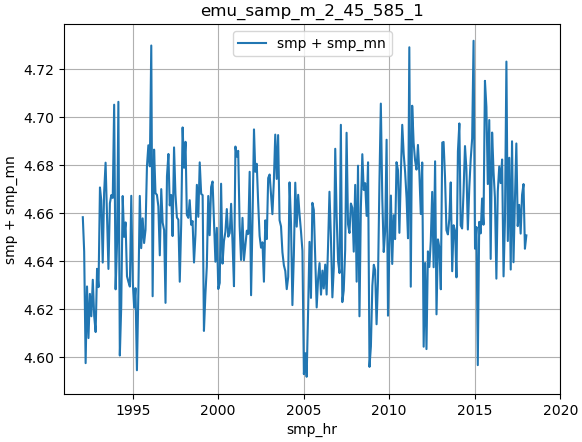
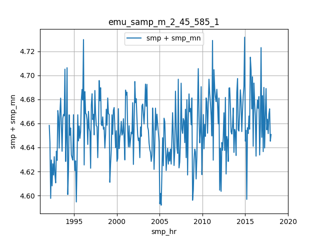
The Sampling (samp) Tool evaluates time-series of the model state. This tutorial describes how to extract V4r4’s monthly mean ocean bottom pressure (OBP) at the North Pole. We will then show how to visualize the results. As specified in EMU Introduction, the extraction is conducted on the P-Cluster, while the visualization is done on OSS.
Run Sampling Tool#
The EMU tools are manually driven and provide straightforward on-screen messages. Nevertheless, we provide detailed commands and their corresponding output below.
Request an interactive node
As described in EMU Introduction, we first request an interactive node to run the Sampling Tool.
salloc --ntasks=2 --ntasks-per-node=2 --partition=sealevel-c5xl-demand --time=01:00:00
The salloc command above requests one node that allows a maximum of two tasks to run in parallel from the partition sealevel-c5xl-demand for one hour of wall clock time. The Sampling Tool is not computationally intensive and normally takes less than 10 minutes to complete.
After the salloc is submitted, we will see the following message:
salloc: Granted job allocation 815
salloc: Waiting for resource configuration
Wait for the node to be ready and the prompt to appear:
salloc: Nodes sealevel-c5xl-demand-dy-c5xlarge-1 are ready for job
owang@ip-10-20-22-69:/efs_ecco/owang/ECCO/EMU/tryout$
The node now is ready, and we can proceed with running the Sampling Tool.
/efs_ecco/ECCO/EMU/emu_userinterface_dir/emu
We will see the following message:
 ******************
  This version of EMU is implemented in Singularity
 ******************

Read from file emu_env.singularity ...
   EMU singularity image: /efs_ecco/ECCO/EMU/emu_dir/emu.sif
   EMU input directory: /efs_ecco/ECCO/EMU/emu_input_dir
   EMU compatible mpiexec: /efs_ecco/ECCO/EMU/emu_dir/ompi/bin/mpiexec
   Command to submit batch job: sbatch
   Number of CPU cores used for MITgcm: 96

 ECCO Modeling Utilities (EMU) Version 1.0a ...
 See /efs_ecco/ECCO/EMU/emu_userinterface_dir/README

*****************************************************************
 This is an alpha version of EMU. Please direct any issues and/or
 questions to Ichiro Fukumori (fukumori@jpl.nasa.gov).
*****************************************************************

Press ENTER key to continue ...
Press ENTER key.
Choose among the following tools ...

  1) Sampling (samp); Evaluates state time-series from model output.
  2) Forward Gradient (fgrd); Computes model's forward gradient.
  3) Adjoint (adj); Computes model's adjoint gradient.
  4) Convolution (conv); Evaluates adjoint gradient decomposition.
  5) Tracer (trc); Computes passive tracer evolution.
  6) Budget (budg); Evaluates budget time-series from model output.
  7) Modified Simulation (msim); Re-runs model with modified input.
  8) Attribution (atrb); Evaluates state time-series by control type.

Enter choice ... (1-8)?
Enter 1 for the Sampling Tool.
choice is 1) Sampling Tool (samp)
See /efs_ecco/ECCO/EMU/emu_userinterface_dir/README_samp

************************************
    EMU Sampling Tool (singularity)
************************************

**** Step 1: Tool Setup
     Running setup_samp.sh

**** Step 2: Specification

By default, tool will sample EMU reference run from state files in directory
/efs_ecco/ECCO/EMU/emu_input_dir/emu_ref/diags

Press ENTER key to continue or enter an alternate directory if sampling another run ... ?
Enter ENTER key to use the default EMU reference run directory.
 ... sampling default EMU reference run.
     Running samp.x
 State will be read from : /inside_alt

Evaluating model time-series ...

 Define objective function (OBJF) ...
 Available VARIABLES are ...
    1) SSH (m)
    2) OBP (equivalent sea level m)
    3) THETA (deg C)
    4) SALT (PSU)
    5) UV (m/s)

   Monthly or Daily mean ... (m/d)?
   (NOTE: daily mean available for SSH and OBP only.)
Enter m to sample monthly means.
   fmd = m
   ==> Sampling MONTHLY means ...

------------------
   Choose OBFJ variable (v in Eq 1 of Guide) # 1 ... (1-5)?
   (Enter 0 to end variable selection)
Enter 2 to choose ocean bottom pressure (OBP; in equivalent sea level meters) as the first objective function (OBJF) variable. In this example, we will only choose one OBJF variable, but EMU allows an OBJF to be a linear combination of multiple OBJF variables (see EMU User Guide for an explanation of OBJF; their Eq. 1).
   OBJF variable  1 is OBP
   Choose either VARIABLE at a point (1) or VARIABLE weighted in space (2) ... (1/2)?
Enter 1 to choose OBP at a point.
   ... OBJF will be a scaled VARIABLE at a point

    i.e., MULT * VARIABLE

Choose horizontal location ...
   Enter 1 to select native grid location (i,j),
      or 9 to select by longitude/latitude ... (1 or 9)?
Enter 1 to select a native grid location – the i, j indices of the ECCO LLC90 compact file format (90, 1170).
   Identify point in native grid ...
   i ... (1-90) ?
Enter 45 for index i.
j ... (1-1170) ?
Enter 585 for index j.
 ...... Chosen point is (i,j) = 45   585
         C-grid is (long E, lat N) =   52.0  89.7
         Depth (m)=  4204.2

   Should value at point be relative to global mean ... (enter 1 for yes)?
Enter 1 to have OBP values at the point be relative to the global mean OBP.
   ... OBJF will be relative to global mean


   Enter scaling factor (alpha in Eq 1 of Guide)... ?
Enter 1 to set the scaling factor to one.
   amult =   1.0000E+00

------------------
   Choose OBFJ variable (v in Eq 1 of Guide) # 2 ... (1-5)?
   (Enter 0 to end variable selection)
Enter 0 to end variable selection. The calculation will start automatically.
Sampling Tool output will be in : emu_samp_m_2_45_585_1

... Done samp setup of data.ecco


**** Step 3: Calculation
     Running do_samp.x
 inputdir read : /inside_alt
 nobjf =            1
Sampling MONTHLY means ...


   Mask file : objf_1_mask_C
   Masks maximum absolute value =   1.0000E+00
         at (i,j) =   45   585
   Masks sum =  -2.5547E-05

********************************************
    Results are in emu_samp_m_2_45_585_1/output
********************************************


EMU interactive execution complete. Wed Oct  2 21:52:34 UTC 2024
At this stage, the sampling tool has completed. As shown above, the results are located in emu_samp_m_2_45_585_1/output.
As shown above, EMU allows users to specify spatial ranges, and it then creates a mask file. It also allows users to specify a mask file for use with the Sampling Tool or other tools. This way, users can provide more complex mask files. In Section Create Mask, we provide a few examples for creating mask files.
Tip
In Section Create Mask, we provide a few examples for creating mask files.
Visualize Sampling Tool Results#
In this section, we demonstrate how to use EMU’s built-in plotting script on OSS to visualize the EMU Sampling Tool results.
Tip
A Jupyter Notebook, samp_viz (after downloading, rename it to samp_viz.ipynb), is provided for users’ convenience. It reproduces the steps and figures described in this visualization tutorial. Users can also add more sophisticated analysis on top of this notebook.
Following OSS Introduction, we first log into OSS and start a Jupyter Notebook session. As shown in samp_viz.ipynb (see Tip above), we have two methods: Method 1 is Menu-driven Input and Method 2 is Argument-driven Input. Method 1 provides a menu for users to input parameters and generate plots. Method 2 takes a list of user-specified arguments, extracts data but skips generating plots, and returns a dictionary containing the data. Using the data in the returned dictionary, users can generate the same plots as in Method 1 and perform additional analysis with the data.
Method 2: Argument-based Input#
The detailed steps for Method 2 can be found in samp_viz.ipynb (see Tip above).
Load modules
import sys
sys.path.append('/efs_ecco/ECCO/EMU/emu_userinterface_dir/')
import emu_plot_arg_py as ept
import numpy as np
import matplotlib.pyplot as plt
Invoke Method 2
globals_dict = ept.emu_plot(run_name="/efs_ecco/owang/ECCO/EMU/tryout/emu_samp_m_2_45_585_1")
Found file: /efs_ecco/ECCO/EMU/emu_userinterface_dir/emu_env.singularity
EMU Input Files directory: /efs_ecco/ECCO/EMU/emu_input_dir

Specified directory of EMU run to examine: /efs_ecco/owang/ECCO/EMU/tryout/emu_samp_m_2_45_585_1

Reading /efs_ecco/owang/ECCO/EMU/tryout/emu_samp_m_2_45_585_1

Reading Sampling Tool output ...

*********************************************
Read variables
   smp: temporal anomaly of sampled variable
   smp_mn: reference time-mean of sampled variable
from file /efs_ecco/owang/ECCO/EMU/tryout/emu_samp_m_2_45_585_1/output/samp.out_312

*********************************************
Read variable
   smp_hr: sample time (hours from 1/1/1992 12Z)
from file /efs_ecco/owang/ECCO/EMU/tryout/emu_samp_m_2_45_585_1/output/samp.step_312

Plotting sampled time-series ...

***********************
EMU variables read as global variables in module global_emu_var (emu); e.g., emu.nx
***********************
cs                  drc                 drf                 dvol3d
dxc                 dxg                 dyc                 dyg
hfacc               hfacs               hfacw               nr
nx                  ny                  rac                 ras
raw                 raz                 rc                  rf
smp                 smp_hr              smp_mn              sn
xc                  xg                  yc                  yg
Extract Data from Return Dictionary
return_vars_dict = globals_dict.get('return_vars')
samp_t = return_vars_dict['time_values']
samp_v = return_vars_dict['variable']
frun_file = return_vars_dict['samp_path']
Make Plot
tmin = int(np.floor(np.min(samp_t))) - 1
tmax = int(np.ceil(np.max(samp_t))) + 1

plt.figure()
plt.plot(samp_t, samp_v, label='smp + smp_mn')
plt.title(frun_file)
plt.xlabel('smp_hr')
plt.ylabel('smp + smp_mn')
plt.xlim(tmin, tmax)
plt.autoscale(axis='y')
plt.grid(True)
plt.legend()

plt.ion()  # Enable interactive mode
plt.show(block=False)  # Show the plot without blocking
Method 2 generates the figure below (also embedded in samp_viz.ipynb), which is the same as the one generated by Method 1.


